After explaining basic noise functions in Part 1 and the idea of node networks in Part 2, we now move on to the first detailed examination of an integral component of our node network system: The expressions, which power the function nodes. For example, take the expression $$x^2+2 x y + y^2$$; if we want to use this expression, our first task is to parse it from the human-readable string representation to a machine representation that is efficient to work with. Once we have created this expression, another natural goal is to evaluate this expression in an efficient way (for example, for $$x = y = 1$$, the result would be $$4$$. Furthermore, there are multiple transformations of interest. There is analytical derivation, i.e. $$\frac{\partial}{\partial x} (x^2+2 x y +y^2) = 2x +2y$$, and there is prediction, which states for example that for inputs in the ranges $$x \in [-1,1], y \in [-1,1]$$, the output is in the range $$[0,4]$$. Furthermore, optimizations to speed up evaluation can also transform the expression into an equivalent, but smaller form, i.e. $$x^2 + y - y~$$ to $$x^2$$.

This article will primarily deal with creating expressions. The other topics will be covered in the context of node networks in general. Evaluation will be explained in depth in Part 4. The transformations mentioned will be featured soon afterwards. Readers who are familiar with compiler construction may already know much of the content in this article, as creating a structure that evaluates an expression given a string is basically what a compiler does as well. However, since our type system is a bit different from that of a standard programming language, the type inference might still be novel to you. Creating an expression from a string is done in multiple steps, as follows:

1. Tokenization
2. Parsing to a tree
3. Type inference

We will now go over these steps in detail.

Tokenization

Tokenization refers to breaking the input string up into groups of characters, the so-called tokens. A token is a logical group of characters, forming a syntactical entity. Furthermore, tokens are annotated with types that reflect a token's meaning. For example, take the following expression:

(4.4+2.66*dot(diag(x),y)-max(z,w))

Tokenizing this expression leads to the following list of tokens:

( [Operator]
4.4 [Value]
+ [Operator]
2.66 [Value]
* [Operator]
dot [Identifier]
( [Operator]
diag [Identifier]
( [Operator]
x [Identifier]
) [Operator]
, [Operator]
y [Identifier]
) [Operator]
- [Operator]
max [Identifier]
( [Operator]
z [Identifier]
, [Operator]
w [Identifier]
) [Operator]
) [Operator]

This tokenization reduces the complexity of the parsing step, since the parser can then handle these discrete units of syntax, and does not have to bother with the string representation.

This string of tokens could be evaluated now by converting it from infix notation to postfix notation via the shunting-yard algorithm, and then using a simple stack-based evaluation. However, our requirements (such as quick evaluation and prediction) are not easily realizable with this simple approach. Therefore, we need a more sophisticated data structure to hold our expression. To fill this data structure, we need to further process these tokens with a parser.

Parsing

The goal of the parsing stage is to obtain an abstract syntax tree (AST) for the tokens. An AST is a data structure that has the basic structure of a tree, with the tokens serving as the nodes for that tree. Taking the expression above for example, the tree that unambiguously identifies this expression is:

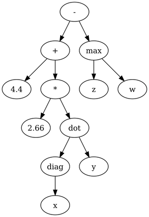
As can be seen from that picture, parentheses and commas are no longer distinct nodes in the tree, since they only provide structure, but no meaning in and of themselves.

To parse the tokens, we implement a simple recursive descent parser. The grammar used for this parser is similar to a simplified portion of the C++ grammar (for "controlling expressions" in the preprocessor), but with a few added features for syntactic sugar described below.

Dot Operator

Instead of calling a function, say clamp, as

clamp(clampee, lower_bound, upper_bound)

we can write

clampee.clamp(lower_bound, upper_bound)

i.e. we take the first parameter and call the function as a pseudo-member function of it. For functions such as clamp, this can provide a greater readability, especially if the arguments are long terms.

Local Variables

A second improvement that helps readability is the ability to use local variables. The syntax is as one would expect from standard imperative languages, i.e.

largeConst = 90000;
dist       = distance2(vec2(0, 0), vec2(x, z));
frac       = largeConst;
frac      /= largeConst+dist;
-100 * frac + y + 90

instead of

-100 * 90000/(90000 + distance2(vec2(0, 0), vec2(x, z))) + y + 90

While using local variables is more verbose, it also enables splitting up long expressions into small, easily understandable chucks. Internally, both representations are parsed to the same AST. In the example with local variables, each variable in the statement is successively replaced by the term on the right hand side of the corresponding assignment.

Type system

Before we can dig into the type inference algorithm, we need to understand the type system used in the expressions. As alluded in the previous article, our type system consists of tensors. A tensor can be understood as a multidimensional array, and every value is a tensor. Scalars are zero-order tensors, vectors are first-order tensors, and matrices are second-order tensors. The order of a tensor determines the number of dimensions that the multidimensional array has, while the dimensions of a tensor specify the sizes of the array's dimensions. A 2x5 matrix is a second-order tensor with the dimensions 2 and 5. (We write [2, 5] for the type). The order of a tensor can be any natural number, and the dimensions can be any natural number that is greater than zero. As a three-dimensional vector can be considered a matrix of dimensions 3x1, it could also be considered a third-order tensor of dimensions [3, 1, 1], or a fourth-order tensor of dimensions [3, 1, 1, 1], and so on. With these tensors, we can now turn to the type inference, which calculates the tensor types for all nodes in our AST.

Type inference

Type inference is executed bottom-up in the AST; since all the leaves have types assigned in the beginning and each operation determines the resulting type from the parameter types, this is straightforward.

The type of a leaf node comes from one of two sources; either the node is a constant, in which case the (tensor-)constant supplies the type, or the node is a variable, in which case the type is taken from the expression's type mapping, which is derived from the expression's context in the node network.

An operation's type transformation can be either a simple transformation, or a complex transformation. A simple transformation assigns one of two possibilities to each input and the output: Scalar($$S$$) or tensor($$T$$). $$S$$ values may only be filled with scalars, $$T~$$ values may be filled with any tensor. However, all $$T~$$ values need to have the same tensor type.

Examples for operations with simple type transformations are:

• the sine has the transformation $$sin(T) = T$$
• addition has the transformation $$T + T = T$$
• dot has the transformation $$dot(T,T) = S$$

If an $$S~$$ is filled with a non-scalar value, this is a type error. However, trying to fill two $$T~$$ with a non-scalar and a scalar value, respectively, is not a type error, since the scalar value can be promoted to a tensor (which will then contain the scalar value in each entry).

A complex transformation is a more specific translation. For example, the diag function creates a diagonal tensor from the argument. In terms of the well-known diagonal matrices, it is a transformation of a type [x] to a type [x, x]. For tensors in general, this leads to the following transformation: $$diag([x, y, z...]) = [x, x, y, z...]$$. This is not expressible with a simple transformation.

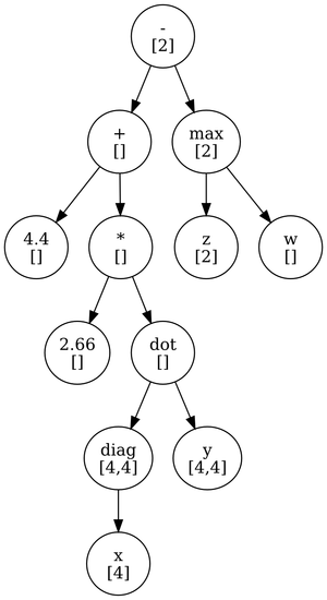
Putting it all together, we can now consider the type inference on the AST given above. Take the following variable types:

x: [4] (vec4)
y: [4,4] (mat4)
z: [2] (vec2)
w: [] (scalar value)

Type inference over the AST yields the following types:

Conclusion

We have seen how expressions are parsed from a string representation into an AST representation via a tokenizer and a parser. Furthermore, we have seen how to infer types on an expression system with tensors as types. The next steps are the evaluation itself, and the various transformations (analytical derivation, range prediction and optimizations), all of which will be detailed over the next few parts in this series.